Omega Group PLC - Pay Discrimination

At the last board meeting of Omega Group Plc., the headquarters of a large multinational company, the issue was raised that women were being discriminated in the company, in the sense that the salaries were not the same for male and female executives. A quick analysis of a sample of 50 employees (of which 24 men and 26 women) revealed that the average salary for men was about 8,700 higher than for women. This seemed like a considerable difference, so it was decided that a further analysis of the company salaries was warranted.
We are asked to carry out the analysis - the objective is to find out whether there is indeed a significant difference between the salaries of men and women, and whether the difference is due to discrimination or whether it is based on another, possibly valid, determining factor.
Import and Inspect
omega <- read_csv(here::here("data", "omega.csv"))
glimpse(omega) # examine the data frame
## Rows: 50
## Columns: 3
## $ salary <dbl> 81894, 69517, 68589, 74881, 65598, 76840, 78800, 70033, 635…
## $ gender <chr> "male", "male", "male", "male", "male", "male", "male", "ma…
## $ experience <dbl> 16, 25, 15, 33, 16, 19, 32, 34, 1, 44, 7, 14, 33, 19, 24, 3…Relationship (Salary - Gender)
The data frame omega contains the salaries for the sample of 50 executives in the company.
We performed two analyses to find out if there is a significant difference between the salaries of the male and female executives - (1) Confidence Intervals and (2) Hypothesis Testing, and see if both lead to the same conclusion.
Two Separate Confidence Intervals
# Summary Statistics of salary by gender
mosaic::favstats (salary ~ gender, data=omega)
## gender min Q1 median Q3 max mean sd n missing
## 1 female 47033 60338 64618 70033 78800 64543 7567 26 0
## 2 male 54768 68331 74675 78568 84576 73239 7463 24 0# Dataframe with two rows (male-female) and having as columns gender, mean, SD, sample size, the t-critical value, the standard error, the margin of error, and the low/high endpoints of a 95% condifence interval
formula_ci_salary <- omega %>%
group_by(gender) %>%
summarise(mean_salary = mean(salary),
sd_salary = sd(salary),
count = n(),
# get t-critical value with (n-1) degrees of freedom
t_critical = qt(0.975, count-1),
se = sd_salary/sqrt(count),
margin_of_error = t_critical * se,
ci_low = mean_salary - margin_of_error,
ci_high = mean_salary + margin_of_error
)
formula_ci_salary %>%
kable() | gender | mean_salary | sd_salary | count | t_critical | se | margin_of_error | ci_low | ci_high |
|---|---|---|---|---|---|---|---|---|
| female | 64543 | 7567 | 26 | 2.06 | 1484 | 3056 | 61486 | 67599 |
| male | 73239 | 7463 | 24 | 2.07 | 1523 | 3151 | 70088 | 76390 |
ggplot(formula_ci_salary,
       aes(x=mean_salary,
           y=gender,
           colour=gender)) +
  geom_point() +
  scale_colour_manual(values = c("red","blue")) +
  geom_errorbar(width=.2, aes(xmax = ci_high, xmin = ci_low)) +
  theme_bw() +
  labs(title = "Which gender has a higher salary?",
       x = "Mean salary",
       y = "Gender") +
  NULL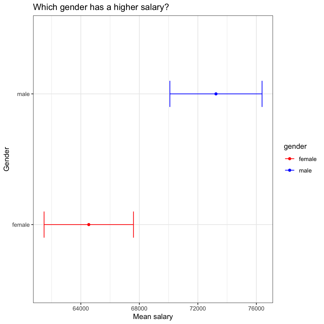
Interpretation: In this analysis, we compared the confidence intervals for the mean salaries of men and women to determine whether the difference between the two means is statistically significant. Based on our analysis, the mean salary for women is 64543, but it can be anywhere between 61486 and 67599. On the other hand, the mean salary for men is 73239, but it can be anywhere between 70088 and 76390. When visualising the two confidence intervals, we can also see that the two does not overlap. Hence, we can conclude that there is a significant difference between the salaries of the men and women executives, where women has a lower average salary than men.
Hypothesis Testing
To perform a hypothesis testing, we assume the null hypothesis (H0) that there is no difference in mean salary between men and women (difference is zero), and the alternative Hypothesis (Ha) that there is a difference in mean salary between men and women (difference is non-zero).
We performed our hypothesis testing using t.test() and with the simulation method from the infer package.
t.test()
mosaic::favstats(salary ~ gender, data = omega)## gender min Q1 median Q3 max mean sd n missing
## 1 female 47033 60338 64618 70033 78800 64543 7567 26 0
## 2 male 54768 68331 74675 78568 84576 73239 7463 24 0t.test(salary ~ gender, data = omega)##
## Welch Two Sample t-test
##
## data: salary by gender
## t = -4, df = 48, p-value = 2e-04
## alternative hypothesis: true difference in means between group female and group male is not equal to 0
## 95 percent confidence interval:
## -12973 -4420
## sample estimates:
## mean in group female mean in group male
## 64543 73239Interpretation: When running the hypothesis test using
t.test(), we get a t-stat value of -4, which is greater than the 5% critical value of 1.96. Another way to look at it is that the CI for the difference between the two means is [-12973, -4420] which does not contains zero. Hence, we can reject the null hypothesis and conclude that there is a significant difference between the salaries of male and female executives.
Simulation Method (infer package)
set.seed(1234)

# calculate the observed statistic
observed_statistic_salary <- omega %>%
  specify(salary ~ gender) %>%
  calculate(stat = "diff in means",
            order = c("male", "female"))

observed_statistic_salary
## Response: salary (numeric)
## Explanatory: gender (factor)
## # A tibble: 1 × 1
## stat
## <dbl>
## 1 8696.# generate the null distribution with randomisation
diff_salary_null_world <- omega %>%
specify(salary ~ gender) %>%
hypothesize(null = "independence") %>%
generate(reps = 1000, type = "permute") %>%
calculate(stat = "diff in means",
order = c("male", "female"))
# visualise the randomisation-based null distribution and test statistic
diff_salary_null_world %>%
visualize() +
shade_p_value(observed_statistic_salary, direction = "two-sided") +
theme_bw() +
labs(title = "Differences in mean salaries between male and female in a hypothetical null world",
subtitle = "Red line shows observed difference in mean salaries",
x = "Difference in mean salaries\n(Male - Female)",
y = "Count") 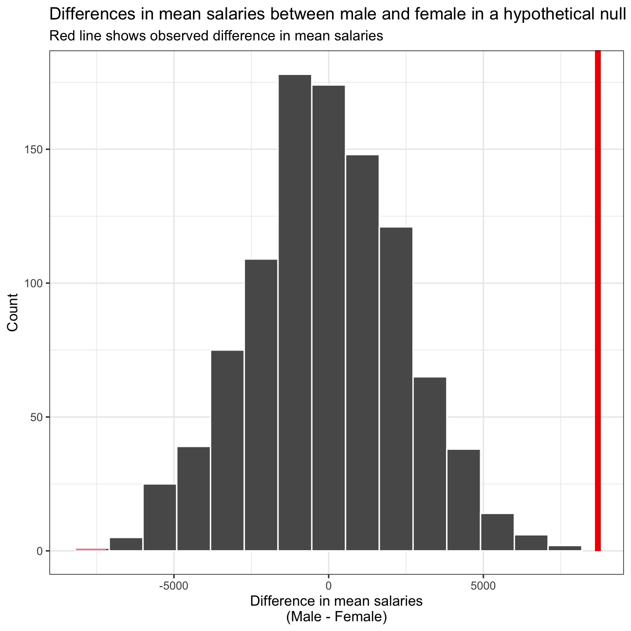
# calculate the p value from the randomisation-based null distribution and the observed statistic
p_value_salary <- diff_salary_null_world %>%
  get_pvalue(obs_stat = observed_statistic_salary,
              direction = "two-sided")

p_value_salary
## # A tibble: 1 × 1
## p_value
## <dbl>
## 1 0Interpretation: Based on our hypothesis testing using the infer package, we get a p-value of close to 0. This means that there’s a close to 0% chance of seeing a difference at least as large as 8696 in a world where there’s no difference. In other words, given what we observed, the null hypothesis is false and it will be impossible to observed such results if the null hypothesis is true. Hence, we can reject the null world and conclude that there is a significant difference between the salaries of male and female executives.
Conclusion
The results of both analyses, comparing both confidence intervals and hypothesis testing, lead to the same conclusion. That is there is a significant difference between the salaries of the male and female executives.
Relationship (Experience - Gender)
At the board meeting, someone raised the issue that there was indeed a substantial difference between male and female salaries, but that this was attributable to other reasons such as differences in experience. A questionnaire send out to the 50 executives in the sample reveals that the average experience of the men is approximately 21 years, whereas the women only have about 7 years experience on average (see table below).
# Summary Statistics of experience by gender
favstats (experience ~ gender, data=omega)
## gender min Q1 median Q3 max mean sd n missing
## 1 female 0 0.25 3.0 14.0 29 7.38 8.51 26 0
## 2 male 1 15.75 19.5 31.2 44 21.12 10.92 24 0Based on this evidence, we performed similar analyses as with the relationship with salary and gender to see if there is a significant difference between the experience of the male and female executives. Let’s see how the conclusion of these analyses validates or endanger our previous conclusion on the difference in male and female salaries.
Two Separate Confidence Intervals
formula_ci_experience <- omega %>%
  group_by(gender) %>%
  summarise(mean_experience = mean(experience),
            sd_experience = sd(experience),
            count = n(),

            # get t-critical value with (n-1) degrees of freedom
            t_critical = qt(0.975, count-1),
            se = sd_experience/sqrt(count),
            margin_of_error = t_critical * se,
            ci_low = mean_experience - margin_of_error,
            ci_high = mean_experience + margin_of_error
            )

formula_ci_experience %>%
kable()| gender | mean_experience | sd_experience | count | t_critical | se | margin_of_error | ci_low | ci_high |
|---|---|---|---|---|---|---|---|---|
| female | 7.38 | 8.51 | 26 | 2.06 | 1.67 | 3.44 | 3.95 | 10.8 |
| male | 21.12 | 10.92 | 24 | 2.07 | 2.23 | 4.61 | 16.52 | 25.7 |
ggplot(formula_ci_experience,
       aes(x=mean_experience,
           y=gender,
           colour=gender)) +
  geom_point() +
  scale_colour_manual(values = c("red","blue")) +
  geom_errorbar(width=.2, aes(xmax = ci_high, xmin = ci_low)) +
  theme_bw() +
  labs(title = "Which gender has more years of experience?",
       x = "Average years of experience",
       y = "Gender") +
  NULL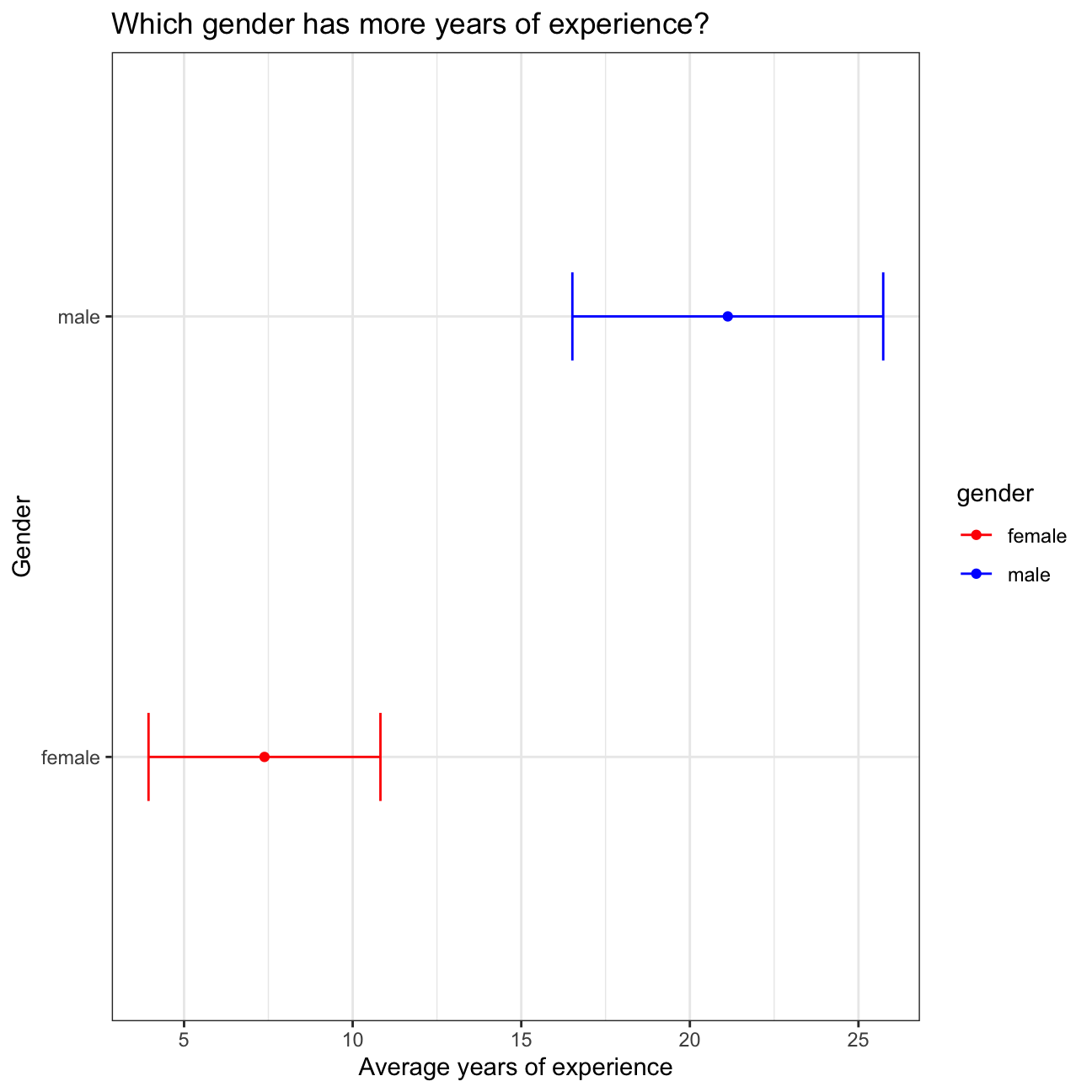
Interpretation: In this analysis, we compared the confidence intervals for the average years of experience of men and women to determine whether the difference between the two means is statistically significant. Based on our analysis, the average years of experience for women is around 7 years, but it can be anywhere between 3.95 and 10.8 years. On the other hand, the average years of experience for men is around 21 years, but it can be anywhere between 16.52 and 25.7 years. When visualising the two confidence intervals, we can also see that the two does not overlap. Hence, we can conclude that there is a significant difference between the experience of the male and female executives, where female have lesser experience than male.
Hypothesis Testing
To perform a hypothesis testing, we assume the null hypothesis (H0) that there is no difference in average experience between men and women (difference is zero), and the alternative Hypothesis (Ha) that there is a difference in average experience between men and women (difference is non-zero).
We performed our hypothesis testing using t.test() and with the simulation method from the infer package.
t.test()
mosaic::favstats(experience ~ gender, data = omega)## gender min Q1 median Q3 max mean sd n missing
## 1 female 0 0.25 3.0 14.0 29 7.38 8.51 26 0
## 2 male 1 15.75 19.5 31.2 44 21.12 10.92 24 0t.test(experience ~ gender, data = omega)##
## Welch Two Sample t-test
##
## data: experience by gender
## t = -5, df = 43, p-value = 1e-05
## alternative hypothesis: true difference in means between group female and group male is not equal to 0
## 95 percent confidence interval:
## -19.35 -8.13
## sample estimates:
## mean in group female mean in group male
## 7.38 21.12Interpretation: When running the hypothesis test using
t.test(), we get a t-stat value of -5, which is greater than the 5% critical value of 1.96. Another way to look at it is that the CI for the difference between the two means is [7.38, 21.12] which does not contains zero. Hence, we can reject the null hypothesis and conclude that there is a significant difference between the experience of the male and female executives.
Simulation Method (infer package)
set.seed(1234)

# calculate the observed statistic
observed_statistic_experience <- omega %>%
  specify(experience ~ gender) %>%
  calculate(stat = "diff in means",
            order = c("male", "female"))

observed_statistic_experience
## Response: experience (numeric)
## Explanatory: gender (factor)
## # A tibble: 1 × 1
## stat
## <dbl>
## 1 13.7# generate the null distribution with randomisation
diff_experience_null_world <- omega %>%
specify(experience ~ gender) %>%
hypothesize(null = "independence") %>%
generate(reps = 1000, type = "permute") %>%
calculate(stat = "diff in means",
order = c("male", "female"))
# visualize the randomisation-based null distribution and test statistic
diff_experience_null_world %>%
visualize() +
shade_p_value(observed_statistic_experience, direction = "two-sided") +
theme_bw() +
labs(title = "Differences in experience between male and female in a hypothetical null world",
subtitle = "Red line shows observed difference in average experience",
x = "Difference in average experience\n(Male - Female)",
y = "Count") 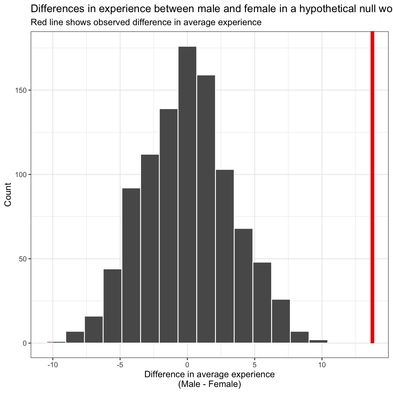
# calculate the p value from the randomisation-based null distribution and the observed statistic
p_value_experience <- diff_experience_null_world %>%
  get_pvalue(obs_stat = observed_statistic_experience,
              direction = "two-sided")

p_value_experience
## # A tibble: 1 × 1
## p_value
## <dbl>
## 1 0Interpretation: Based on our hypothesis testing using the infer package, we get a p-value of close to 0. This means that there’s a close to 0% chance of seeing a difference at least as large as 13.7 years in a world where there’s no difference. In other words, given what we observed, the null hypothesis is false and it will be impossible to observed such results if the null hypothesis is true. Hence, we can reject the null world and conclude that there is a significant difference between the experience of the male and female executives.
Conclusion
The results of both analyses, comparing both confidence intervals and hypothesis testing, led to the same conclusion. That is there is a significant difference between the experience of the male and female executives.
Relationship (Salary - Experience)
Someone at the meeting argues that clearly, a more thorough analysis of the relationship between salary and experience is required before any conclusion can be drawn about whether there is any gender-based salary discrimination in the company.
Hence, we drew a scatter plot to visually inspect the data and analysed the relationship between salary and experience.
Salary vs Experience Scatter Plot
# Calculating Pearson's product-moment correlation
cor.test(omega$experience, omega$salary, method = "pearson", conf.level = 0.95)
##
## Pearson's product-moment correlation
##
## data: x and y
## t = 9, df = 48, p-value = 2e-12
## alternative hypothesis: true correlation is not equal to 0
## 95 percent confidence interval:
## 0.676 0.884
## sample estimates:
## cor
## 0.803ggplot(omega, aes(x = experience, y = salary)) +
geom_point() +
geom_smooth(method = lm, col = "red") +
labs(title = "The relationship between salary and experience",
x = "Years of experience",
y = "Salary") +
theme_bw() +
annotate("text", x = 5, y = 85000, col = "red", size = 6,
label = paste("Pearson r = ", signif(cor(omega$experience, omega$salary),3))) 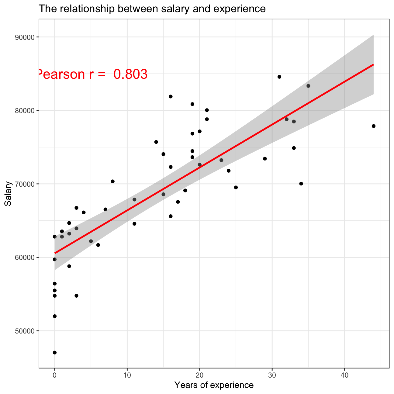
NULL## NULLCheck correlations between the data
We used GGally:ggpairs() to create a scatter plot and correlation matrix. Essentially, we change the order of our variables will appear in and have the dependent variable (Y), salary, as last in our list. We then pipe the data frame to ggpairs() with aes arguments to colour by gender and make these plots somewhat transparent (alpha = 0.3).
omega %>%
  select(gender, experience, salary) %>% #order variables they will appear in ggpairs()
  ggpairs(aes(colour=gender, alpha = 0.3))+
  theme_bw()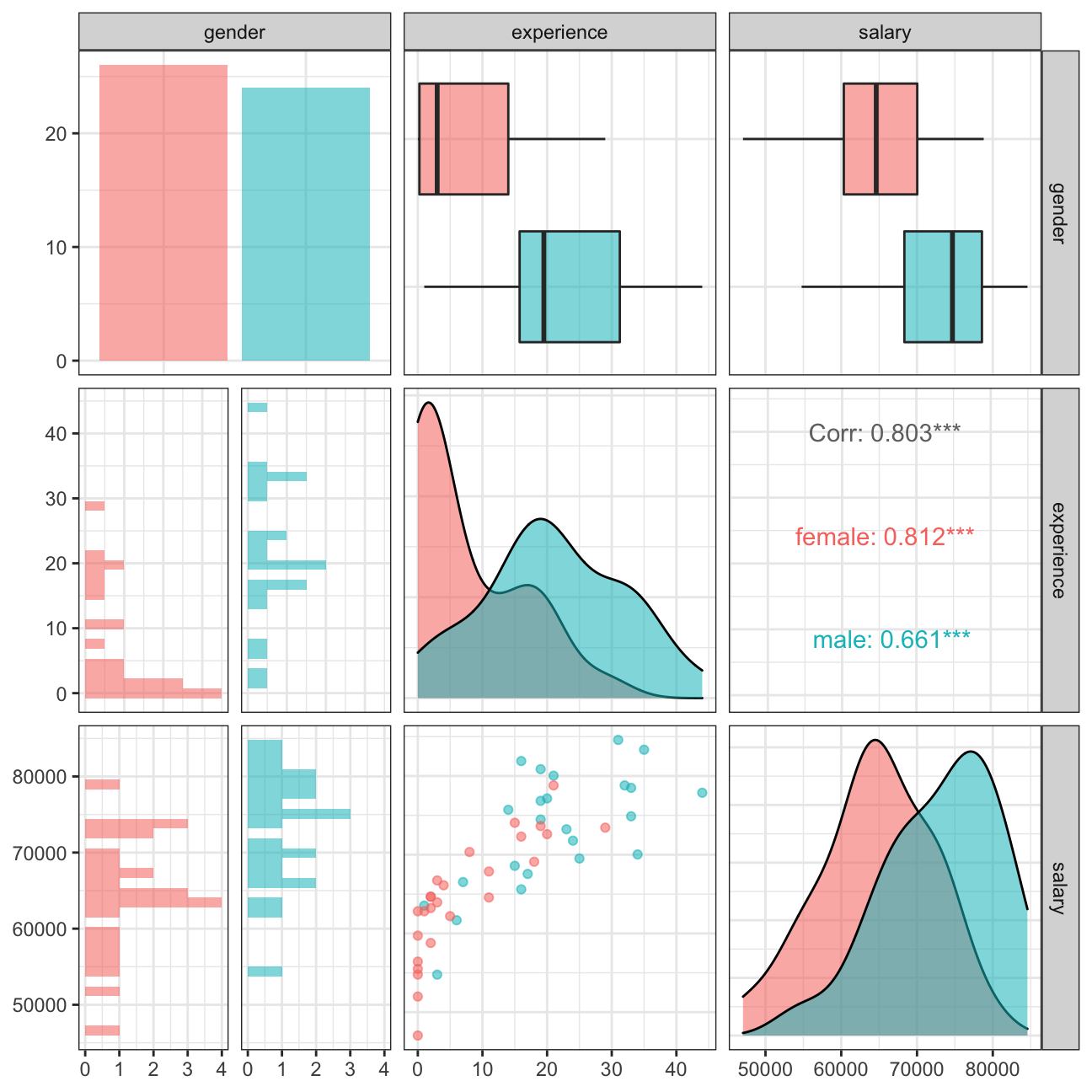
Interpretation: Based on our analysis, there is a positive relationship between salary and experience as the correlation coefficient is close to 1. In other words, as years of experience increases, salary increases. When categorizing the gender into different colors, we can see that more women are on the left side of the graph, indicating lesser years of experience on average. Hence, this is a good indication as of why women has a lower average salary as compared to men.
Final conclusion
According to our analysis, there is a positive relationship between salary and experience, and women has lower years of experience than men on average. Hence, the assumption that women were being discriminated in the company in the sense that the salaries were not the same for male and female executives may not be true. The substantial difference between male and female salaries is more likely attributable to differences in experience.