IMDb Movie Database Analysis

The subset sample of movies is taken from the Kaggle IMDB 5000 movie dataset
Import and Inspect
movies <- read_csv(here::here("data", "movies.csv"))
glimpse(movies)
## Rows: 2,961
## Columns: 11
## $ title <chr> "Avatar", "Titanic", "Jurassic World", "The Avenge…
## $ genre <chr> "Action", "Drama", "Action", "Action", "Action", "…
## $ director <chr> "James Cameron", "James Cameron", "Colin Trevorrow…
## $ year <dbl> 2009, 1997, 2015, 2012, 2008, 1999, 1977, 2015, 20…
## $ duration <dbl> 178, 194, 124, 173, 152, 136, 125, 141, 164, 93, 1…
## $ gross <dbl> 7.61e+08, 6.59e+08, 6.52e+08, 6.23e+08, 5.33e+08, …
## $ budget <dbl> 2.37e+08, 2.00e+08, 1.50e+08, 2.20e+08, 1.85e+08, …
## $ cast_facebook_likes <dbl> 4834, 45223, 8458, 87697, 57802, 37723, 13485, 920…
## $ votes <dbl> 886204, 793059, 418214, 995415, 1676169, 534658, 9…
## $ reviews <dbl> 3777, 2843, 1934, 2425, 5312, 3917, 1752, 1752, 35…
## $ rating <dbl> 7.9, 7.7, 7.0, 8.1, 9.0, 6.5, 8.7, 7.5, 8.5, 7.2, …Besides the obvious variables of title, genre, director, year, and duration, the rest of the variables are as follows:
gross: the gross earnings in the US box office, not adjusted for inflationbudget: the movie’s budgetcast_facebook_likes: the number of facebook likes cast members receivedvotes: the number of people who voted for (or rated) the movie in IMDBreviews: the number of reviews for that movierating: IMDB average rating
Check for missing values (NAs) and if all entries are distinct
skimr::skim(movies)| Name | movies |
| Number of rows | 2961 |
| Number of columns | 11 |
| _______________________ | |
| Column type frequency: | |
| character | 3 |
| numeric | 8 |
| ________________________ | |
| Group variables | None |
Variable type: character
| skim_variable | n_missing | complete_rate | min | max | empty | n_unique | whitespace |
|---|---|---|---|---|---|---|---|
| title | 0 | 1 | 1 | 83 | 0 | 2907 | 0 |
| genre | 0 | 1 | 5 | 11 | 0 | 17 | 0 |
| director | 0 | 1 | 3 | 32 | 0 | 1366 | 0 |
Variable type: numeric
| skim_variable | n_missing | complete_rate | mean | sd | p0 | p25 | p50 | p75 | p100 | hist |
|---|---|---|---|---|---|---|---|---|---|---|
| year | 0 | 1 | 2.00e+03 | 9.95e+00 | 1920.0 | 2.00e+03 | 2.00e+03 | 2.01e+03 | 2.02e+03 | ▁▁▁▂▇ |
| duration | 0 | 1 | 1.10e+02 | 2.22e+01 | 37.0 | 9.50e+01 | 1.06e+02 | 1.19e+02 | 3.30e+02 | ▃▇▁▁▁ |
| gross | 0 | 1 | 5.81e+07 | 7.25e+07 | 703.0 | 1.23e+07 | 3.47e+07 | 7.56e+07 | 7.61e+08 | ▇▁▁▁▁ |
| budget | 0 | 1 | 4.06e+07 | 4.37e+07 | 218.0 | 1.10e+07 | 2.60e+07 | 5.50e+07 | 3.00e+08 | ▇▂▁▁▁ |
| cast_facebook_likes | 0 | 1 | 1.24e+04 | 2.05e+04 | 0.0 | 2.24e+03 | 4.60e+03 | 1.69e+04 | 6.57e+05 | ▇▁▁▁▁ |
| votes | 0 | 1 | 1.09e+05 | 1.58e+05 | 5.0 | 1.99e+04 | 5.57e+04 | 1.33e+05 | 1.69e+06 | ▇▁▁▁▁ |
| reviews | 0 | 1 | 5.03e+02 | 4.94e+02 | 2.0 | 1.99e+02 | 3.64e+02 | 6.31e+02 | 5.31e+03 | ▇▁▁▁▁ |
| rating | 0 | 1 | 6.39e+00 | 1.05e+00 | 1.6 | 5.80e+00 | 6.50e+00 | 7.10e+00 | 9.30e+00 | ▁▁▆▇▁ |
There are no missing values as can be observed when analysing
n_missing. However, there are duplicate values for some variables. What is more likely our concern is that there are duplicate titles, which shouldn’t be the case. This can be observed through looking atn_unique: even though there are a total of 2961 records, there only seem to be 2907 unique movie titles.
Number of movies in each genre
count_movies_genre <- movies %>%
  group_by(genre) %>%
  count(sort=TRUE) %>%
  rename("number of movies" = n)

count_movies_genre
## # A tibble: 17 × 2
## # Groups: genre [17]
## genre `number of movies`
## <chr> <int>
## 1 Comedy 848
## 2 Action 738
## 3 Drama 498
## 4 Adventure 288
## 5 Crime 202
## 6 Biography 135
## 7 Horror 131
## 8 Animation 35
## 9 Fantasy 28
## 10 Documentary 25
## 11 Mystery 16
## 12 Sci-Fi 7
## 13 Family 3
## 14 Musical 2
## 15 Romance 2
## 16 Western 2
## 17 Thriller 1There is a significant difference between the genre with the highest number of movies - Comedy, and the genre with the lowest number of movies - Thriller.
Return on budget - how much $ did a movie make at the box office for each $ of its budget
library(scales)

genre_returns <- movies %>%
  group_by(genre) %>%
  summarise(average_gross = mean(gross),
            average_budget = mean(budget)) %>%
  mutate(return_on_budget = average_gross/average_budget) %>%
  mutate(return_on_budget = round(return_on_budget, 2)) %>%
  mutate(average_gross = dollar(average_gross), average_budget = dollar(average_budget)) %>%
  # The dollar function is from the scales package which allows the numbers to be more readable

  arrange(desc(return_on_budget))

genre_returns
## # A tibble: 17 × 4
## genre average_gross average_budget return_on_budget
## <chr> <chr> <chr> <dbl>
## 1 Musical $92,084,000 $3,189,500 28.9
## 2 Family $149,160,478 $14,833,333 10.1
## 3 Western $20,821,884 $3,465,000 6.01
## 4 Documentary $17,353,973 $5,887,852 2.95
## 5 Horror $37,713,738 $13,504,916 2.79
## 6 Fantasy $42,408,841 $17,582,143 2.41
## 7 Comedy $42,630,552 $24,446,319 1.74
## 8 Mystery $67,533,021 $39,218,750 1.72
## 9 Animation $98,433,792 $61,701,429 1.6
## 10 Biography $45,201,805 $28,543,696 1.58
## 11 Adventure $95,794,257 $66,290,069 1.45
## 12 Drama $37,465,371 $26,242,933 1.43
## 13 Crime $37,502,397 $26,596,169 1.41
## 14 Romance $31,264,848 $25,107,500 1.25
## 15 Action $86,583,860 $71,354,888 1.21
## 16 Sci-Fi $29,788,371 $27,607,143 1.08
## 17 Thriller $2,468 $300,000 0.01Top 15 directors who have created the highest gross revenue in the box office
top_directors <- movies %>%
  group_by(director) %>%
  summarise(total_gross = sum(gross),
            avg_gross = mean(gross),
            median_gross = median(gross),
            sd_gross = sd(gross)) %>%
  slice_max(order_by = total_gross, n = 15) %>%
  mutate(total_gross = dollar(total_gross),
         avg_gross = dollar(avg_gross),
         median_gross = dollar(median_gross),
         sd_gross = dollar(sd_gross))

top_directors
## # A tibble: 15 × 5
## director total_gross avg_gross median_gross sd_gross
## <chr> <chr> <chr> <chr> <chr>
## 1 Steven Spielberg $4,014,061,704 $174,524,422 $164,435,221 $101,421,051
## 2 Michael Bay $2,231,242,537 $171,634,041 $138,396,624 $127,161,579
## 3 Tim Burton $2,071,275,480 $129,454,718 $76,519,172 $108,726,924
## 4 Sam Raimi $2,014,600,898 $201,460,090 $234,903,076 $162,126,632
## 5 James Cameron $1,909,725,910 $318,287,652 $175,562,880 $309,171,337
## 6 Christopher Nolan $1,813,227,576 $226,653,447 $196,667,606 $187,224,133
## 7 George Lucas $1,741,418,480 $348,283,696 $380,262,555 $146,193,880
## 8 Robert Zemeckis $1,619,309,108 $124,562,239 $100,853,835 $91,300,279
## 9 Clint Eastwood $1,378,321,100 $72,543,216 $46,700,000 $75,487,408
## 10 Francis Lawrence $1,358,501,971 $271,700,394 $281,666,058 $135,437,020
## 11 Ron Howard $1,335,988,092 $111,332,341 $101,587,923 $81,933,761
## 12 Gore Verbinski $1,329,600,995 $189,942,999 $123,207,194 $154,473,822
## 13 Andrew Adamson $1,137,446,920 $284,361,730 $279,680,930 $120,895,765
## 14 Shawn Levy $1,129,750,988 $102,704,635 $85,463,309 $65,484,773
## 15 Ridley Scott $1,128,857,598 $80,632,686 $47,775,715 $68,812,285Ratings distribution
ratings_by_genre <- movies %>%
  group_by(genre) %>%
  summarise(avg_rating = mean(rating),
           min_rating = min(rating),
           max_rating = max(rating),
           sd_rating = sd(rating)) %>%
  arrange(desc(avg_rating))

ratings_by_genre
## # A tibble: 17 × 5
## genre avg_rating min_rating max_rating sd_rating
## <chr> <dbl> <dbl> <dbl> <dbl>
## 1 Biography 7.11 4.5 8.9 0.760
## 2 Crime 6.92 4.8 9.3 0.849
## 3 Mystery 6.86 4.6 8.5 0.882
## 4 Musical 6.75 6.3 7.2 0.636
## 5 Drama 6.73 2.1 8.8 0.917
## 6 Documentary 6.66 1.6 8.5 1.77
## 7 Sci-Fi 6.66 5 8.2 1.09
## 8 Animation 6.65 4.5 8 0.968
## 9 Romance 6.65 6.2 7.1 0.636
## 10 Adventure 6.51 2.3 8.6 1.09
## 11 Family 6.5 5.7 7.9 1.22
## 12 Action 6.23 2.1 9 1.03
## 13 Fantasy 6.15 4.3 7.9 0.959
## 14 Comedy 6.11 1.9 8.8 1.02
## 15 Horror 5.83 3.6 8.5 1.01
## 16 Western 5.7 4.1 7.3 2.26
## 17 Thriller 4.8 4.8 4.8 NA# Plotting the graph that shows how ratings are distributed (all genres)
ggplot(movies, aes(x=rating)) +
geom_histogram(color="black", fill = "grey") +
geom_vline(aes(xintercept=mean(rating)), color = "darkred", size = 1, linetype = "dashed") +
labs(title = "Ratings distribution",
subtitle = "A histogram on overall ratings across genres",
x = "Rating",
y = "count") +
annotate("text",
label = "Mean",
color = "darkred",
y = -10,
x = 7,
size = 5) +
theme_bw() 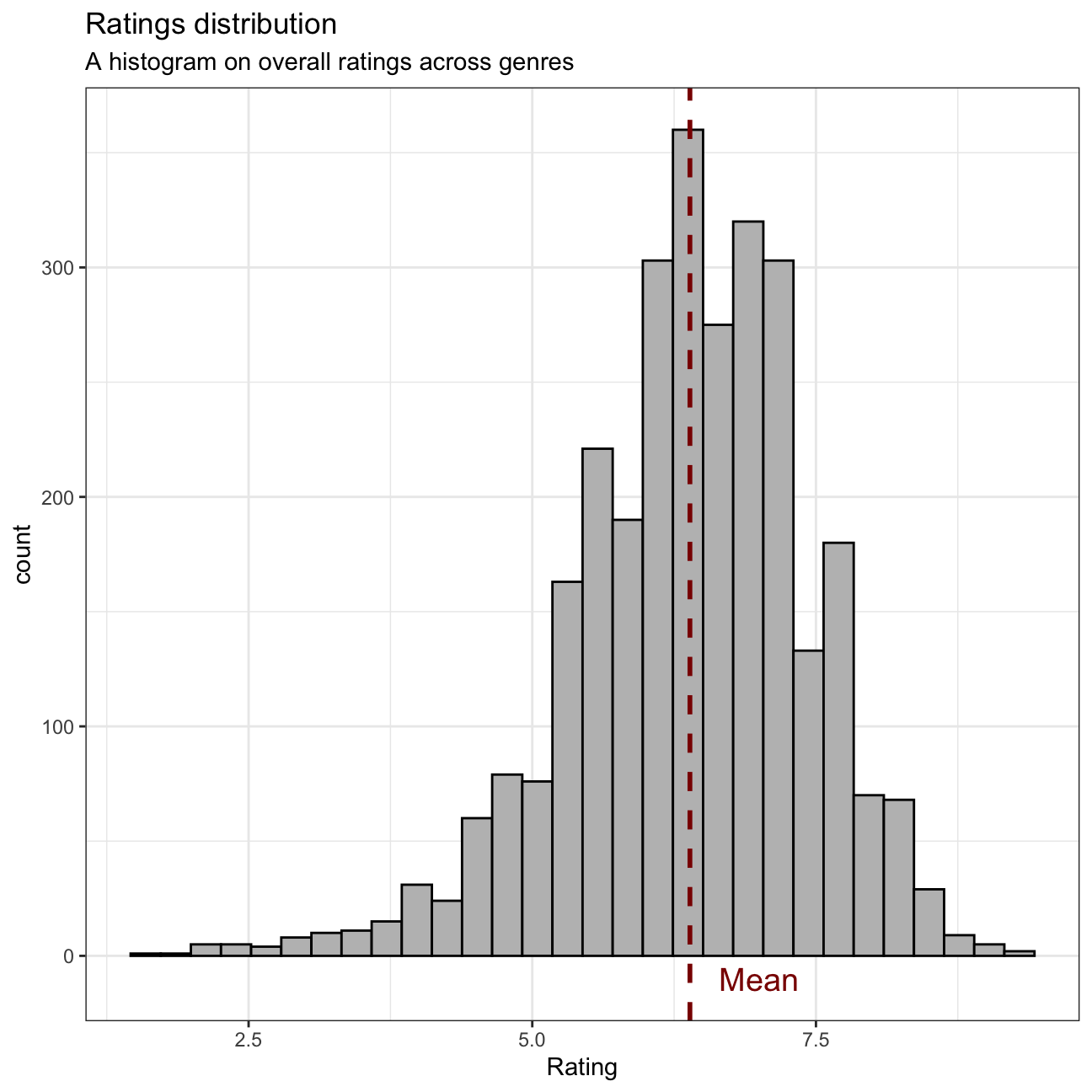
# Plotting the graph that shows how ratings are distributed by genre
ggplot(movies, aes(x=rating)) +
  geom_histogram(color="black", fill = "grey") +
  facet_wrap(vars(genre), scales = "free_y") +
  labs(title = "Ratings distribution by genre",
         x = "Rating") +
  theme_bw()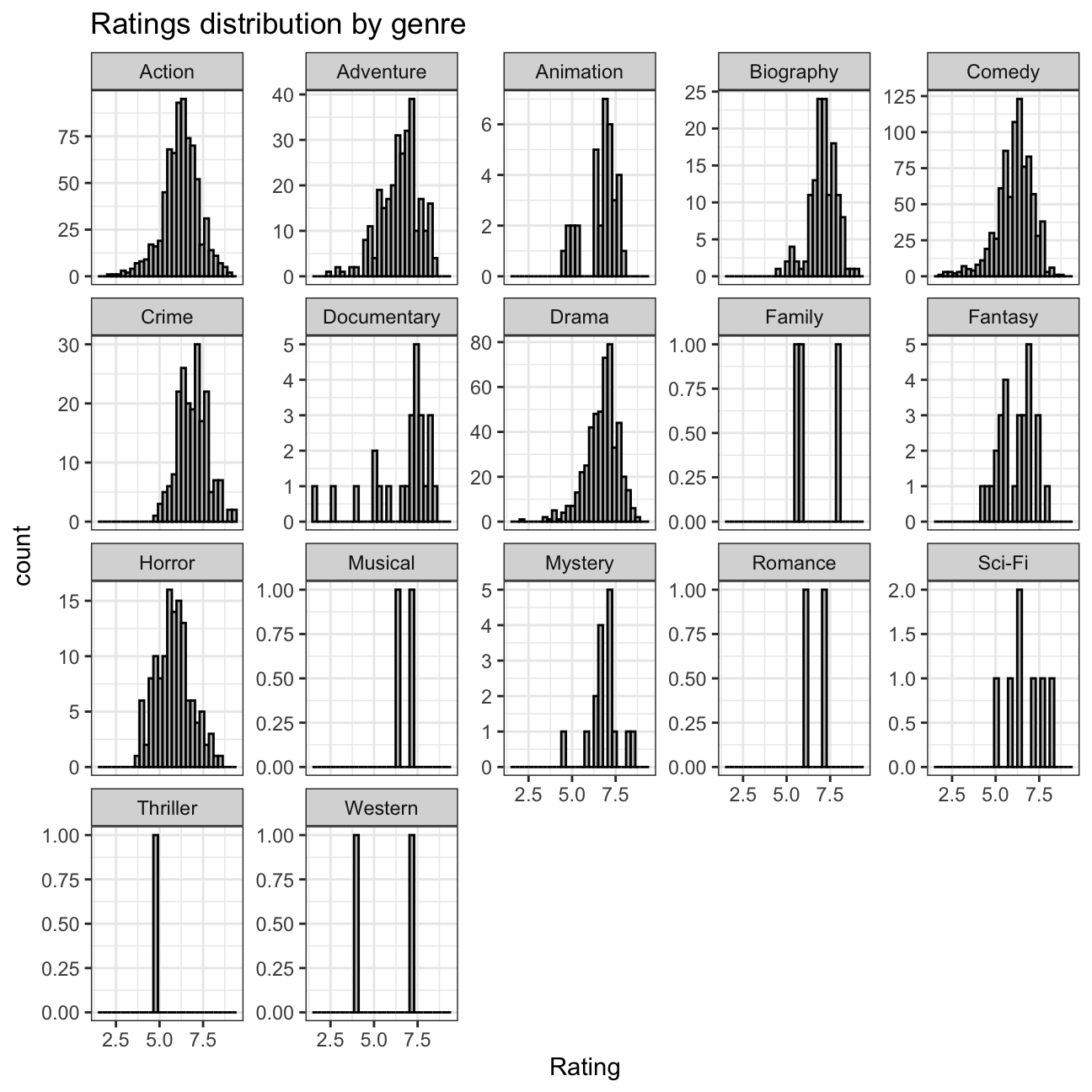
The relationship between gross and cast_facebook_likes
We would like to find out if the number of facebook likes that the casts have received is likely to be a good predictor of how much money a movie will make at the box office.
ggplot(movies, aes(x=cast_facebook_likes, y=gross)) +
  geom_point(aes(color=genre)) +
  geom_smooth(method = "lm") +
  labs(title = "Casts' Facebook likes and gross revenue",
       subtitle = "The relationship between casts' Facebook popularity and the movie's gross revenue (Unadjusted)",
       x = "Casts' likes on facebook",
       y = "Gross revenue") +
  stat_regline_equation(label.x = 50000, label.y = 760000000, aes(label = ..eq.label..), size = 3) +
  stat_regline_equation(label.x = 50000, label.y = 730000000, aes(label = ..rr.label..), size = 3) +
  scale_x_continuous(labels = number) +
  scale_y_continuous(labels = dollar_format(prefix = "$", suffix = "m", scale = 1/1000000))+
  theme_bw()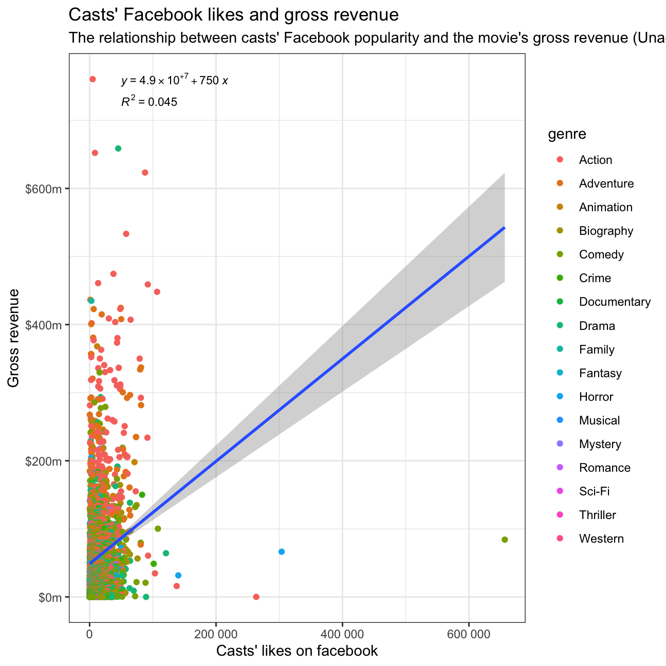
#Removing outliers to improve visualisation

ggplot(movies, aes(x=cast_facebook_likes, y=gross)) +
  geom_point(aes(color=genre)) +
  geom_smooth(method = "lm") +
  xlim(0, 150000) + #Limiting the display of values on the x and y axes to account for outliers
  ylim(0,600000000) +
  labs(title = "Casts' Facebook likes and gross revenue",
       subtitle = "The relationship between casts' Facebook popularity and the movie's gross revenue (Adjusted)",
       x = "Casts' likes on facebook",
       y = "Gross revenue") +
  stat_regline_equation(label.x = 15000, label.y = 750000000, aes(label = ..eq.label..), size = 3) +
  stat_regline_equation(label.x = 15000, label.y = 730000000, aes(label = ..rr.label..), size = 3) +
  scale_y_continuous(labels = dollar_format(prefix = "$", suffix = "m", scale = 1/1000000))+
theme_bw()-1.png)
From the R2 value of 0.081, we can infer that the correlation between the two variables is rather weak. This indicates that the casts’ Facebook popularity does not solely help to predict the gross revenue of a movie.
The relationship between gross and budget
We would like to find out if the budget for the movie is likely to be a good predictor of how much money the movie will make at the box office.
ggplot(movies, aes(x=budget, y=gross)) +
  geom_point(aes(color=genre)) +
  geom_smooth(method = "lm") +
  labs(title = "Movie budget and gross revenue",
       subtitle = "The relationship between the movie's budget and its' gross revenue",
       x = "Budget",
       y = "Gross revenue") +
  stat_regline_equation(label.y = 700000000, aes(label = ..eq.label..), size = 3) +
  stat_regline_equation(label.y = 670000000, aes(label = ..rr.label..), size = 3) +
  scale_x_continuous(labels = dollar_format(prefix = "$", suffix = "m", scale = 1/1000000))+
  scale_y_continuous(labels = dollar_format(prefix = "$", suffix = "m", scale = 1/1000000))+
  theme_bw()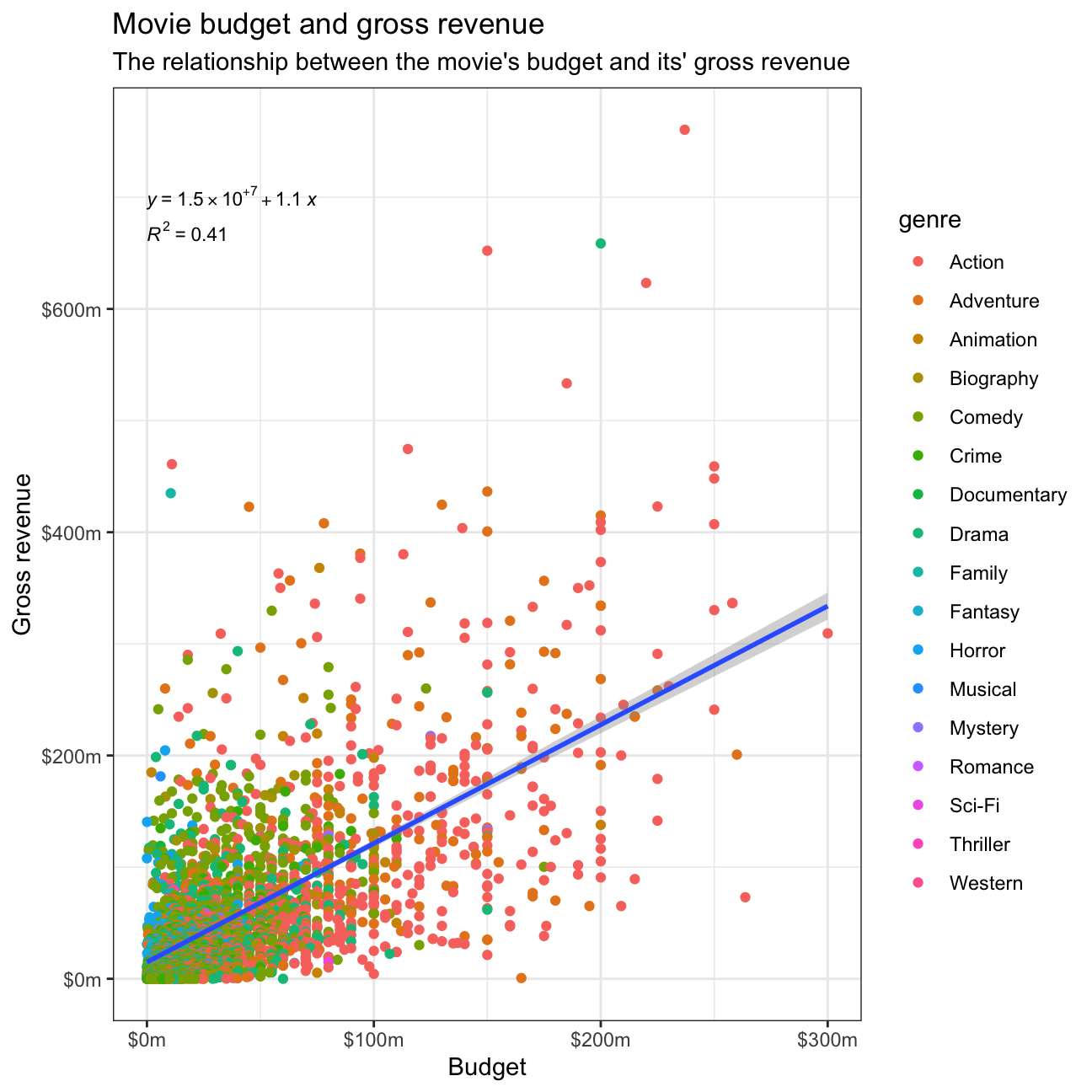
Budget seems to be a stronger predictor of a movie’s gross revenue compared to casts’ facebook popularity, as the R2 value is closer to 1.
The relationship between gross and rating
We would like to find out whether IMDB ratings are likely to be a good predictor of how much money a movie will make at the box office
ggplot(movies, aes(x=rating, y=gross)) +
  geom_point(aes(color=genre), size=1) +
  geom_smooth(method = "lm") +
  scale_x_continuous(labels = number) +
  scale_y_continuous(labels = dollar) +
  labs(title = "Movie rating and gross revenue",
       subtitle = "The relationship between the movie's rating and its' gross revenue",
       x = "Rating",
       y = "Gross revenue") +
  stat_regline_equation(label.y = 700000000, aes(label = ..eq.label..), size = 3) +
  stat_regline_equation(label.y = 670000000, aes(label = ..rr.label..), size = 3) +
  scale_y_continuous(labels = dollar_format(prefix = "$", suffix = "m", scale = 1/1000000)) +
  theme_bw()


# Faceted by genre
ggplot(movies, aes(x=rating, y=gross)) +
  geom_point(aes(color=genre), size=0.5) +
  geom_smooth(method = "lm") +
  facet_wrap(vars(genre), scale="free_y") +
  scale_x_continuous(labels = number) +
  scale_y_continuous(labels = dollar) +
  labs(title = "Movie rating and gross revenue",
       subtitle = "The relationship between the movie's rating and its' gross revenue",
       x = "Rating",
       y = "Gross revenue") +
  facet_wrap(vars(genre), scale="free_y") +
  scale_y_continuous(labels = dollar_format(prefix = "$", suffix = "m", scale = 1/1000000)) +
  theme_bw()
In general, there is a positive correlation between a movie’s rating and its gross revenue. However, similar to casts’ Facebook likes, the correlation is weak. Other than that, due to the small sample size of some genres (e.g Musical, Western and Sci-Fi), not all trendlines are representative.